Data-center build gauge
An early-warning gauge for the semiconductor cycle
The whole semiconductor ecosystem rides on data-center buildout, and chips are bought near the end of a build. So the job is to measure how fast data centers are actually being built, watch the leading edge of the pipeline, and turn that into a forward read on AI-chip demand. Two builds of the same idea below — pick the tab.
MVP The lean gauge
The smallest build that delivers the signal: a monthly read on the data-center build rate as an early warning for AI-chip demand. It stands on published trackers plus a short list of high-signal sources — no project-level database, no scraping fleet.
Is the build rate accelerating, steady, or decelerating — and what does that imply for semiconductors over the next 2–4 quarters?
US + the top ~10 global markets, quarterly, aggregate GW kept separate by basis. North-America-heavy, transparent markets only.
Reuse Knight Frank / JLL / Sightline / Goldman aggregates, a few utility interconnection queues, and hyperscaler capex. Compute the flow + one lead/lag check.
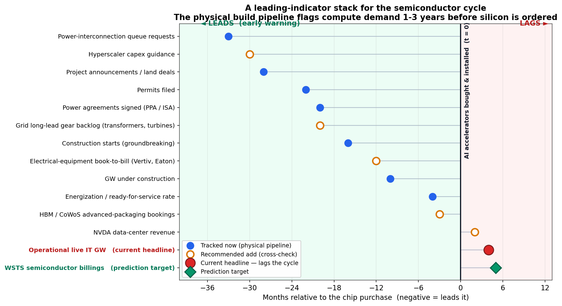
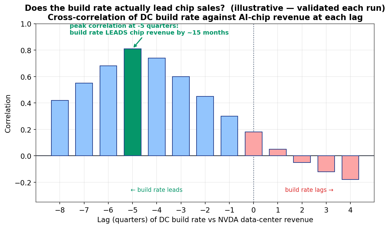
A one-page dashboard: regime banner, build-rate chart, the indicator ladder, a lead/lag check, a track record (past forecast vs realized), and a one-paragraph read.

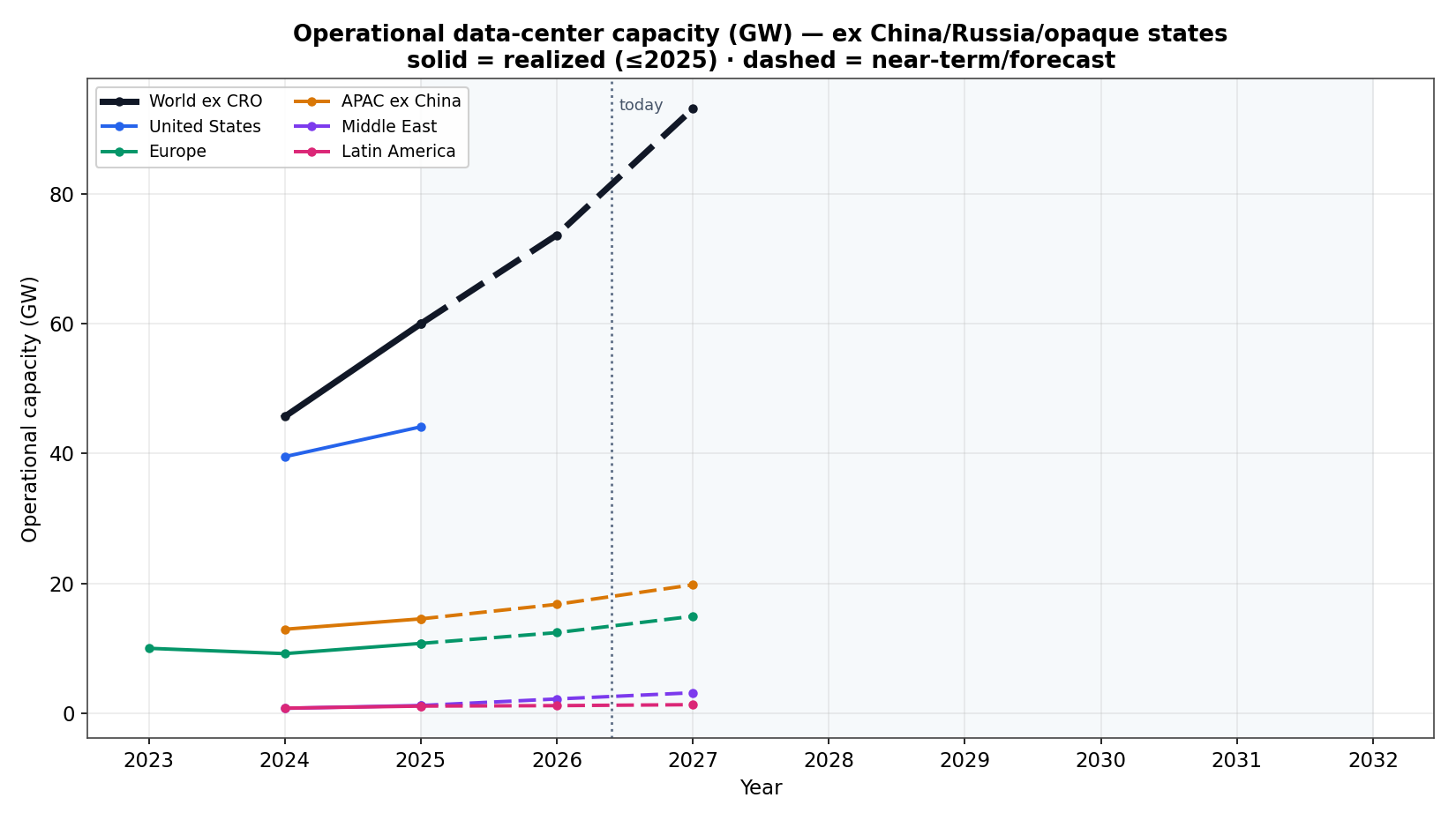
The build rate — the leading flow, not the finished stock — with a plain regime verdict on top. This single chart is the MVP's core deliverable.
Why MVP first. This captures roughly 80% of the signal for about 10% of the effort, and — critically — it lets us test whether the build rate actually leads chip sales before investing in the full pipeline. If the lead holds, the Expansive build is justified; if not, we re-anchor cheaply.
MVP How the lean gauge runs — build spec
A monthly, resumable pipeline of five steps. A few agents, a fixed source list, and one SQLite file that every agent writes to as it works — so you can watch the run fill in live. This panel is the spec; it is detailed enough to hand to another agent and have it build the thing.
📄 Full implementation spec → BUILD_MVP.md (hand this to an agent)The five steps
Architecture at a glance
One SQLite file (WAL mode) is the whole data store — inspectable, and WAL lets a progress view read while agents write. Sources live in a registry + one adapter per source; the pipeline never special-cases a source. Agents are thin: read from the DB, write to the DB, update their progress row.
# repo layout — the source + extraction library
gauge/
  run.py                # orchestrator (python -m gauge.run)
  db/ schema.sql conn.py gauge.db
  sources/
    registry.yaml       # seeds the `sources` table
    base.py             # Extractor ABC + Observation
    capital_intent/  market_tracker/
    power_queue/     equipment/  target/
  extractors/ normalize.py  llm.py
  pipeline/ gather.py extract.py reconcile.py
            compute.py publish.py
  progress/ app.py  progress.html
  templates/ gauge.html.j2
  charts/  raw/
Agents write to the DB as they progress (real-time)
run_steps is the single source of truth for progress. Each step sets its row to running before work and done/error after, with a live rows_written count and a per-source sub-row. A tiny Flask view (or a polled progress.json) renders the step tree, updating every 3s while the run executes.
-- the live progress feed (DDL excerpt)
CREATE TABLE run_steps (
  run_id  TEXT, step TEXT,
  unit    TEXT DEFAULT '-',   -- source_id or '-'
  agent   TEXT,
  status  TEXT,               -- pending|running|done|error
  started_at TEXT, ended_at TEXT,
  rows_written INTEGER DEFAULT 0,
  message TEXT,
  PRIMARY KEY (run_id, step, unit)
);
// GET /api/progress?run_id=2026-06
{
  "run": {"status":"running","current_step":"extract"},
  "steps": [
    {"step":"gather","unit":"-","status":"done","rows_written":12},
    {"step":"gather","unit":"knight_frank","status":"done"},
    {"step":"extract","unit":"ercot_queue","status":"running"},
    {"step":"compute","unit":"-","status":"pending"}
  ]
}
Full schema (9 tables: runs · run_steps · sources · raw_documents · observations · series · metrics · regime_calls · review_queue) is in the spec. The regime_calls table is the seed of the track record — one logged call per run.
Step contracts
| Step | Agent | Reads | Writes | Done when |
|---|---|---|---|---|
| 1 · gather | Gather agent | sources (enabled) | raw_documents, run_steps[unit=source] | every source has a raw doc or error |
| 2 · extract | Extraction agent | raw_documents | observations, review_queue | all docs parsed or queued |
| 3 · reconcile | Reconcile fn | observations | series | required metrics populated |
| 4 · compute | Compute agent | series | metrics, regime_calls | regime + lead/lag present |
| 5 · publish | Publish fn | metrics, series, regime_calls | charts/*.png, gauge.html | files written |
Resumable: a step is skipped if its run_steps row is done for the run. --only <source> re-runs one source; --resume <run_id> continues a crashed run.
The source & extraction library
Every source implements one interface, so the extraction agent never branches per source. Two kinds behind it: structured (FMP API / CSV / HTML table → deterministic) and document (PDF / press release → schema-locked LLM extraction that must keep the source snippet). Add a source = add a registry row + a parser class.
# sources/base.py — the one interface
@dataclass
class Observation:
    metric: str      # operational_capacity | capex | ...
    region: str
    basis: str       # it_load | grid_demand | capex_usd ...
    period: str      # 2025 | 2025Q4 | 2026-05
    value: float; unit: str       # GW | USD_bn
    confidence: str  # verified|strongly|weakly
    snippet: str     # exact source text (audit)

class Extractor:
    source_id: str; family: str
    def fetch(self) -> RawDoc: ...
    def parse(self, raw) -> list[Observation]: ...
| Source | Family | Basis | Lead | Kind |
|---|---|---|---|---|
| MSFT / AMZN / GOOGL / META / ORCL capex | capital_intent | capex $ | ~10 q | FMP |
| Knight Frank | market_tracker | IT load | coincident | doc/LLM |
| JLL · Cushman | market_tracker | IT load | ~2 q | doc/LLM |
| Sightline Climate | market_tracker | IT load | ~6 q | doc/LLM |
| Goldman US activations | market_tracker | IT load | ~4 q | doc/LLM |
| ERCOT · PJM queues | power_queue | grid | ~11 q | PDF/XLSX |
| Vertiv book-to-bill | equipment | grid | ~4 q | transcript/LLM |
| NVDA data-center revenue | target | revenue $ | lagging | FMP |
Compute definitions & run
No-ambiguity definitions
build_rate_gw_q = quarterly net additions of the promoted World-ex-CRO IT-load series. regime = accelerating if YoY of the 4-q trailing avg > +10%, decelerating if < −10%, else steady. lead/lag = argmax cross-correlation of build rate vs NVDA DC revenue; < 8 overlapping quarters ⇒ confidence low. Thresholds live in config.py.
# run it
python -m gauge.run                # current month
python -m gauge.run --month 2026-06
python -m gauge.run --only ercot_queue
python -m gauge.run --resume 2026-06
python -m gauge.progress           # live view :8090

# build order: schema → conn → base+registry
# → 2 FMP extractors (nvda, msft) → gather
# → extract → reconcile → compute → publish
# → progress view → remaining extractors
Bases never averaged together. Only same-publisher / same-basis pairs count as forecast revisions. Every figure carries a source + confidence + snippet; the regime call carries a confidence tag. Idempotent per month; series upserts.
No per-project database, no permit scraping, no satellite, no cohort stage-tracking, no global long-tail. Those are the Expansive build — added only once the lead is proven.
MVP The one-page gauge
Everything the MVP ships fits on one screen: the verdict, the chart behind it, which signals it watched, and whether the lead holds. Example run, June 6 2026.

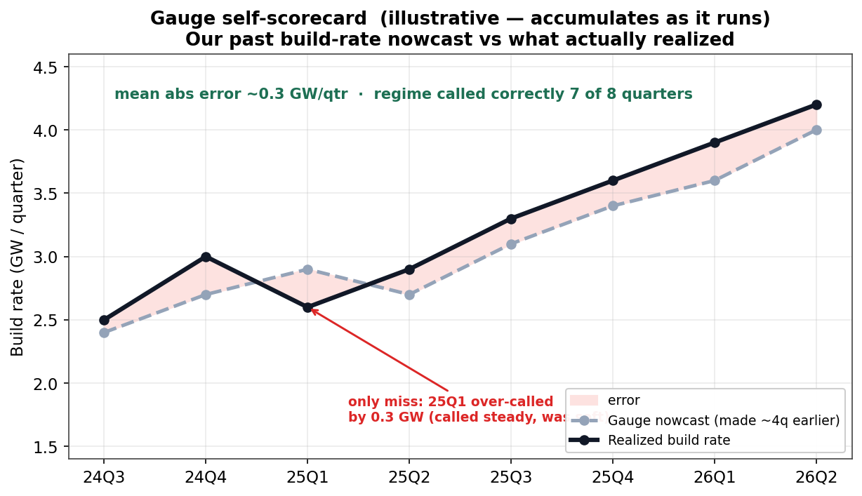
The 2025 forecast (55.6 GW) came in low — actual was 60.0 GW. Forecasts have run ~5–8% below realized, so the gauge tags confidence medium and treats the current call as, if anything, conservative. This is what earns the regime call the right to be believed.
This run's read. Net additions are running ~4.2 GW/quarter and still climbing; every leading layer (power-queue requests, hyperscaler capex, construction starts) is rising in step. The build rate has historically led NVDA data-center revenue by ~5 quarters, so the signal points to continued AI-chip demand strength into 2027. Confidence is medium — the AI-era history is short, so treat the lead as directional, not precise.
Expansive The full leading-indicator engine
The same idea, taken all the way: every layer of the indicator stack, global coverage, down to project-level stage tracking — with backtested lead/lag per indicator, a GW→dollar bridge, scenario forecasts, and a defensible audit trail. This turns the gauge from a read into a forecasting engine with attribution.
Interconnection queues across every major ISO/utility (ERCOT, PJM, AESO, Dominion, Georgia Power…), energization rates, and request withdrawals — the earliest and hardest-to-fake signal.
Permit filings, satellite-detected construction starts, and grid long-lead-equipment backlogs (transformers, turbines) — what's actually happening on the ground.
A stage_transitions table records each project's stage at every snapshot → real conversion rates, dwell-time, and RFS schedule adherence.
A silicon-intensity model (HBM / CoWoS / ASP per MW) converts the physical build rate into an AI-chip-dollar demand nowcast.
Per-indicator backtested lead/lag, a forecast-accuracy scorecard (incl. the gauge grading its own past calls), and a clear answer each run to "which layer flashed first?"
Low / base / high build-rate fans, global coverage including long-tail markets, and human-review queues for ambiguous records.

Why expand. The aggregate trackers the MVP relies on update slowly and are pre-digested. Project-level tracking catches a slowdown earlier — as stalls, slipping RFS dates, and queue withdrawals — and it can attribute the move to a layer. The cost is real: a continuous multi-agent pipeline and a data layer that only gets accurate as it ages.
Expansive How the full engine runs
A continuous, resumable, Codex-driven multi-agent pipeline writing to a database. Charts, the API, and the regime call regenerate on every run; the project/event/stage layer accumulates over time.
stage_transitions, dwell-time, slippage, capacity reconcile.resolver + confidenceSource families
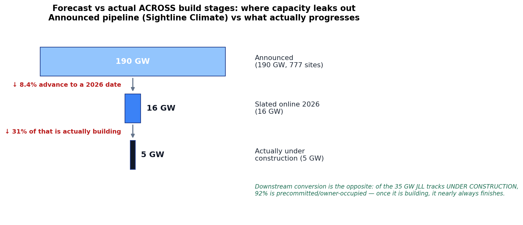
A stage_transitions table — every project's stage at each snapshot. This is what makes longitudinal forecast-vs-actual possible: of the capacity under construction last quarter, how much actually hit its forecast RFS date?
Cohort accumulation takes time to become accurate; satellite construction detection is noisy; the silicon-intensity model needs maintenance; and the lead/lag has a short AI-era history → confidence bands stay wide and are stated, not hidden.
Cadence: continuous / weekly, fully resumable so a run can be killed and resumed without losing the data store. Cost scales with the source-family fan-out; the QA queues keep a human in the loop where confidence is low.
Expansive The full chart pack + forecasting engine
The complete output: the levels and build rate, the forecast-vs-actual evidence, the leading-indicator panel with attribution, and the GW→$ nowcast. Example run, June 6 2026.


Track record — past forecast vs realized
The scoreboard. Third-party forecasts vs what landed, and — the gold standard — the gauge grading its own past calls. Both feed the confidence bands on every forward number.
| Forecaster | Target | Predicted | Realized / current | Miss |
|---|---|---|---|---|
| Knight Frank (2025 vintage) | 2025 live IT GW | 55.6 | 60.0 | −7.3% (under) |
| Knight Frank (2025 vintage) | 2026 live IT GW | 66.5 | 73.6* | −9.7% (under) |
| Goldman (scheduled) | US 2025 activations | — | 8.5 realized | fills in as years realize |
| This gauge (self-scorecard) | build-rate regime | 7 / 8 correct | MAE ~0.3 GW/qtr | accumulates each run |
*current estimate, not yet fully realized. The project-level version of this is RFS schedule adherence (forecast RFS date vs actual) — see the spec tiles below.
Per-indicator lead/lag & current reading
| Indicator | Typical lead | Reading this run | Confidence |
|---|---|---|---|
| Power-interconnection requests | ~11 q | rising sharply | Low–med |
| Hyperscaler capex guidance | ~10 q | rising | High |
| Construction starts | ~5 q | rising | Med |
| Electrical-equipment book-to-bill | ~4 q | > 1, rising | Med |
| GW under construction | ~3 q | rising | High |
| HBM / CoWoS bookings | ~1 q | sold out | Med |
Charts still on the spec (need the stage layer)
Per-cohort stage-to-stage conversion rates over time — needs the stage_transitions history.
How long capacity sits in each stage, and whether that's lengthening (an early stall signal).
Forecast RFS date vs actual RFS date — true schedule slippage, the cleanest project-level forecast-vs-actual.
This run's read. Every layer of the stack is rising in step, and the earliest layer — power-interconnection requests — flashed first, which is the most leading signal we have. The build rate leads NVDA data-center revenue by ~5 quarters, and the GW→$ bridge says chip dollars rise faster than GW because intensity is climbing. Net: AI-chip demand strength looks well-supported into 2027, with the usual caveat that scheduled activations carry delay/cancellation risk concentrated in the steep 2027 slate.